Data_Reduction_Manual
Last-modified: 2019-09-13 (金) 18:48:29 (1688d)
Top / Data_Reduction_Manual
NIC Data Reduction Manual
Abstract †
- Here we present the reduction procedures of imaging data (w/o polarimetry) obtained with NIC.
- The data are assumed to be obtained with the procedures shown in the Observers' Manual
- This document is based on the article below:
- In modifying and editing the article, some materials provided by J. Takahashi were used.
- You can use a set of the pipeline scripts working on the host 'gamera' (192.168.42.204), which automatically reduces the raw data (not accessible from outside the NHAO).
The scheme of the data reduction †
- The data reduction is outlined as follows. The names of the automatically-generated files in each step are shown in the parenthesis.
- Dark subtraction (*.da.fits)
- Flatfielding (*.fl.fits)
- Mask and interpolate the bad pixels
- Mask and interpolate the hot pixels and dark pixels (*.rr.fits)
- Generate the sky frame (*.sk.fits)
- Subtract the sky frame (*.ss.fits)
- Subtract the 'stripe' pattern of the detector (*.sp.fits)
- Match the positions by shifting the individual frames
- Coadd the frames to generate the combined image (*.cm.fits)
- Register and assign the WCS to the combined frame (*.cmw.fits)
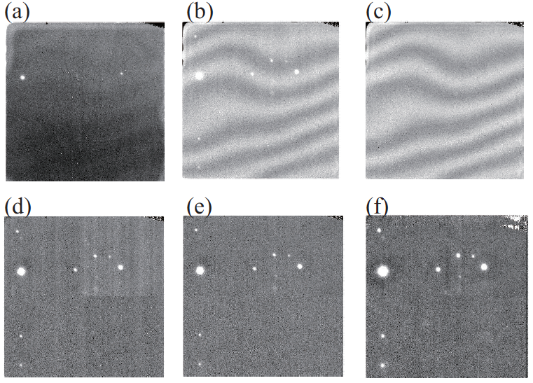
- The figure above shows the example image generated in each step. (a) Raw image, (b) The image after the step 4, (c) The sky frame generated in the step 5, (d) Sky-subtracted image after the step 6, (e) The 'stripe'-subtracted image after step 7, (f) The final image
1. Dark subtraction †
- Use the dark frames obtained by the procedure shown here.
- Be sure to set the exposure time for the dark frames exactly the same as that for the object frame.
- Obtain 10-15 frames, and coadd them to generate the dark frame.
- The pipeline scripts installed in 'gamera' performs 3-sigma clipping, then averages the remaining frames.
- If the cold shutter is not set to the appropriate position, some unexpected light comes into the frame. Be sure to remove such frames before running the scripts.
- Subtract the coadded dark frame from the object frames (and also the flat frames).
- The pipeline script generates the intermediate file named *.da.fits. The example below is for J band.
After dark-subtraction j(date)_(frameID).(ObjectName).da.fits [e.g., j120717_0098.SN2012dn_01.da.fits]
2. Flatfielding †
- This step corrects for the spatial inhomogeneity of the sensitivity.
- Usually we recommend to use the twilight flat. This link (Japanese) explains how to obtain the flat frames.
- If you use the master flat frames provided by the observatory, find the frames at the nearest date in the directory gamera:/home/nhao/nic/nicred.latest/common/.
- We do not have any specially-made software tools to generate flat frames. The only NIC-specific features are those shown in the link above.
- How to generate a flat frame is outlines as follows:
- Obtain 5-10 (or more) pairs of flat frames with high- and low counts. The difference between the high- and low-count frames should be at least ~2000.
- Subtract the low-count frame from the high-count frame for each pair.
- Homogenise the count levels by scale the individual frames with the median counts, and coadd them. (e.g., use IRAF/images.immatch.imcombine with combine=median, scale=median, reject=avsigclip)
- Normalise the coadded frame so as to set the average count to be unity. (e.g., use IRAF/noao.imred.generic.normalize)
- Divide the dark-subtracted frame with the normalised flat frame. (e.g., use IRAF/images.imutil.imarith)
- The pipeline script generates the intermediate file named *.fl.fits (below is an example for J band).
After flatfielding j(date)_(frameID).(ObjectName).fl.fits [e.g., j120717_0098.SN2012dn_01.fl.fits]
3 & 4. Mask and interpolate the bad pixels and the hot/dark pixels †
- Bad pixels (appear at fixed positions) can be removed by using, e.g., IRAF/proto.fixpix.
- The table shown below are the lists of bad pixels for J-, H- and K bands. The format is "x1 x2 y1 y2", i.e., for each line,
- Mask the region with x1<x<x2, y1<y<y2, and interpolate the pixel values using the pixels around that region.
- If there are only two columns, mask only the single pixel and interpolate using the pixels surrounding the masked pixel.
- J band
277 291 134 148
186 191 229 236
260 270 1017 1023
- H band
277 291 134 148
186 191 229 236
961 962 672 673
1002 1004 652 654
1005 1006 649 651
966 967 612 619
964 966 609 614
1001 1007 646 654
13 15 242 245
- K band
140 141 549 551
162 163 806 807
162 805
163 804
164 167 801 803
162 170 795 800
171 173 798 802
186 191 229 236
277 291 134 148
320 321 586 589
321 323 591 593
778 779 682 688
780 786 671 676
779 780 677 680
785 789 670 671
- Hot/dark pixels can be removed using, e.g., IRAF/noao.imred.crutil.cosmicrays. For dark pixels, multiply the whole image with -1 and do the same thing.
cosmicrays @obj_fl.lst @obj_cr1.lst
imarith @obj_cr1.lst * -1 @obj_cr2.lst
cosmicrays @obj_cr2.lst @obj_cr3.lst
imarith @obj_cr3 * -1 @obj_cr4.lst

 obj_fl.lst:    list of the flatfielded files
 obj_cr?.lst: list of files to be generated
- The recommended parameters for IRAF/cosmicrays are: threshold>(5sigma of the sky fluctuation), fluxratio~2-10.
- You can use other tools such as L.A.Cosmic
- The pipeline script generates the files named *.rr.fits (below is an example for J band)
After removing Bad/Hot/Dark pixel j(date)_(frameID).(ObjectName).rr.fits [e.g., j120717_0098.SN2012dn_01.rr.fits]
5 & 6. Sky subtraction †
- The 'sky' here means 'winding' pattern that cannot be corrected even with the dark-subtraction and flatfielding. The procedures shown here subtracts such pattern.
- Step 5. The sky frames are generated by median-stacking the frames obtained in a set of dithering without matching the positions. (e.g., using IRAF/imcombine)
- If the stars are not so crowded, you can use the raw object frames.
- If there are many stars within the FoV, you need to obtain the sky frame containing not so many stars, but as close to the target field as possible. Make sure you use the same read-out mode and exposure time.
- The sky frame can be used even when containing several stars within the FoV.
- The procedures are outlined below. (This is not the only way. NOT necessarily the best way)
- Normalise each sky frame to the median pixel value.
- Median-stack the normalised frames. (e.g., using IRAF/imcombine with scale='median', combine='median', reject='avsigclip')
- Estimate the sky level of each object frame, and scale the sky frame to set the sky counts to the same level.
- Step 6. The sky subtraction is done by simply subtracting the scaled sky frame from the object frame. (e.g., using IRAF/imarith)
- The pipeline scripts generate the following two kinds of files, named *.sk.fits and *.ss.fits (below is an example for J band)
Sky frame generated    j(ObjectName).sk.fits  [e.g., jSN2012dn_01.sk.fits]
Sky-subtracted image  j(date)_(frameID).(ObjectName).ss.fits [e.g., j120717_0098.SN2012dn_01.ss.fits]
7. 'Stripe'-pattern subtraction †
- The NIC imaging data have 'stripe' pattern coming from the detectors. At this point you need to subtract the pattern from the frames.
- This pattern is thought to be due to the voltage fluctuation that cannot be removed with the dark-subtraction and flatfielding.
- The amplitude of this pattern is almost constant for each column, at least during each dithering set. This is unlikely to the 'sky' mentioned above.
- There are two ways of subtraction as follows.
- For sparse fields, i.e., fields containing few stars (Sampling method)
- Extract 20-100 lines without any stars, and average along the y-axis to obtain the 'stripe' pattern profile.
- Do the same procedure for both the upper- and lower halves.
- Subtract the 'stripe' pattern profile of the upper half from the upper half of the object frame,and vice versa.
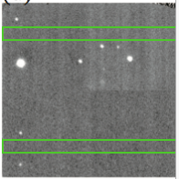
- In the example above the regions outlined with the green boxes are used to obtain the 'stripe'-pattern profiles. The upper box region is used to obtain the upper-half profile of the 'stripe' pattern, and the lower box is used to obtain the lower-half profile.
- For crowded fields, i.e., fields containing many stars (Median method)
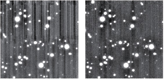
- The example below has many stars in the FoV, and 'lines without stars' cannot be extracted.
- Calculate the median count for each column for each of upper- and lower half, and generate the 'stripe' pattern profile for each half.
- Subtract the profile from the object frames, similarly to the sampling method described above.
- The example above shows the result of subtraction with median method. The left panel shows the object frame before subtraction, and the right panel shows that after subtraction. The 'stripe' pattern is sufficiently well subtracted, although not so good as the results of sampling method.
- The pipeline scripts generate the files named *.sp.fits (below is an example for J band)
After subtracting the 'stripe' pattern j(date)_(frameID).(ObjectName).sp.fits [e.g., j120717_0098.SN2012dn_01.sp.fits]
- The pipeline scripts also try to register the WCS at this point, and generate the files named *.spw.fits, if successful.
8 & 9. Position matching & stacking †
- Measure the positions of astrometric reference stars . (e.g., using IRAF/imexamine, SExtractor, etc.)
- Shift the images so that the reference stars are located at the very same pixel coordinates. (e.g., using IRAF/images.imgeom.imshift)
- You do not need to take account of distortion, as the FoV of NIC is not so wide.
- The position angle is usually set to be constant, so that you do not need to consider the rotation.
- You can utilise the whole FoV of NIC by creating larger-format, blank frame (the counts is et to, e.g., -10000) and pasting the object frame onto it before shifting & stacking. The pipeline scripts do so as default.
- Stack the object frames after matching the positions (e.g., using IRAF/imcombine).
- The pipeline scripts generates the files shown below, named *.sf.fits and *.cm.fits (shown here is an example for J band).
After matching   j(date)_(frameID).(ObjectName).sf.fits  [e.g., j120717_0098.SN2012dn_01.sf.fits]
After Stacking   j(ObjectName).cm.fits  [e.g., jSN2012dn_01.cm.fits]
10. Astrometry †
- Obtain the coordinate system using the stars within the FoV, refering to the 2MASS catalogue, etc. (e.g., using IRAF/imcoords.ccmap, ccsetwcs)
- ccmap : Reads the list of object coordinates and corresponding world coordinates of the stars within the FoV, i.e., list of "X Y RA Dec".
- ccsetwcs : Inputs the 'image to be registered the WCS' and 'output file of ccmap', and outputs the WCS-registered image.
- This is not the only way to do this. You can also use astrometry.net, etc.
- See also: WCSTools
- The pipeline script uses 'imwcs' of WCSTools, and register the WCS based on the 2MASS catalogue. You can run the following commands on 'gamera' to do the astrometry only. (Note that the WCS registering process sometimes fails.)
gamera% ds9 &
gamera% getwcs.sh [file name].cm.fits
- Note that the script does not run on machines other than gamera.
- The script generates the following files named *.spw.fits and *.cmw.fits (below is an example for J band).
After 'stripe' subtraction + WCS     j(date)_(frameID).(ObjectName).spw.fits [e.g.,  j120717_0098.SN2012dn_01.spw.fits]
After stacking + WCS     j(ObjectName).cmw.fits [e.g., jSN2012dn_01.cmw.fits]
- The astrometry process includes the calculation of the pixel scale, and writing it in the FITS header. If the values in the header are very different from 0.16 arcsec/pix, the astrometry is possibly unsuccessful.
Revision history †
- 2019.09.10 Created based on the Japanese version (T. Saito)
- 2019.09.12 Fully revised and opened for public (T. Saito)
添付ファイル:


